A strong association with a broad mapping interval
The report follows the full path from repeated plot observations and imputed HapMap genotypes to mixed-model association, local LD, and positional candidate genes. Its central result is a chromosome 3 association in this breeding panel, with independent validation and finer mapping still needed.
Which genomic regions are associated with flowering time across field trials?
Can flowering-time associations be detected after accounting for trial conditions, genotype × environment variation, relatedness, and population structure in an inbred rice breeding panel?
The phenotype was FL, days to 50% heading. Wet- and dry-season observations from 2009–2012 were combined through a trial-aware mixed model so that repeated plots informed a line estimate rather than being treated as independent genotypes in GWAS.
| Source | User-supplied archives whose exact filenames are listed in Dryad dataset 10.5061/dryad.7369p, associated with Spindel et al. (2015) and the IRRI irrigated rice breeding population. |
|---|---|
| Genotypes | MET_crfilt_.75_allchrom.hmp.txt.zip — imputed HapMap SNP calls |
| Phenotypes | RYT_plotdata_by_GHID_corrected_PUBLIC_ACCESS.zip — plot records from eight year-season trials |
| Reference | Nipponbare MSU v6.0 throughout; matching GFF3 and TU brief annotations |
| Analysis unit | 349 breeding lines after matching and sample QC |
The source publication by Spindel et al. (2015) studied genomic selection and association mapping in elite tropical rice breeding lines. Dryad documents these phenotype files as wet- and dry-season measurements from 2009–2012. The publication's 363-line, 73,147-marker analysis and this session's 349-line, 69,833-marker GWAS use different analysis sets; the present case study does not claim to reproduce the published model or results exactly.
From plot-level records to a kinship-aware association scan
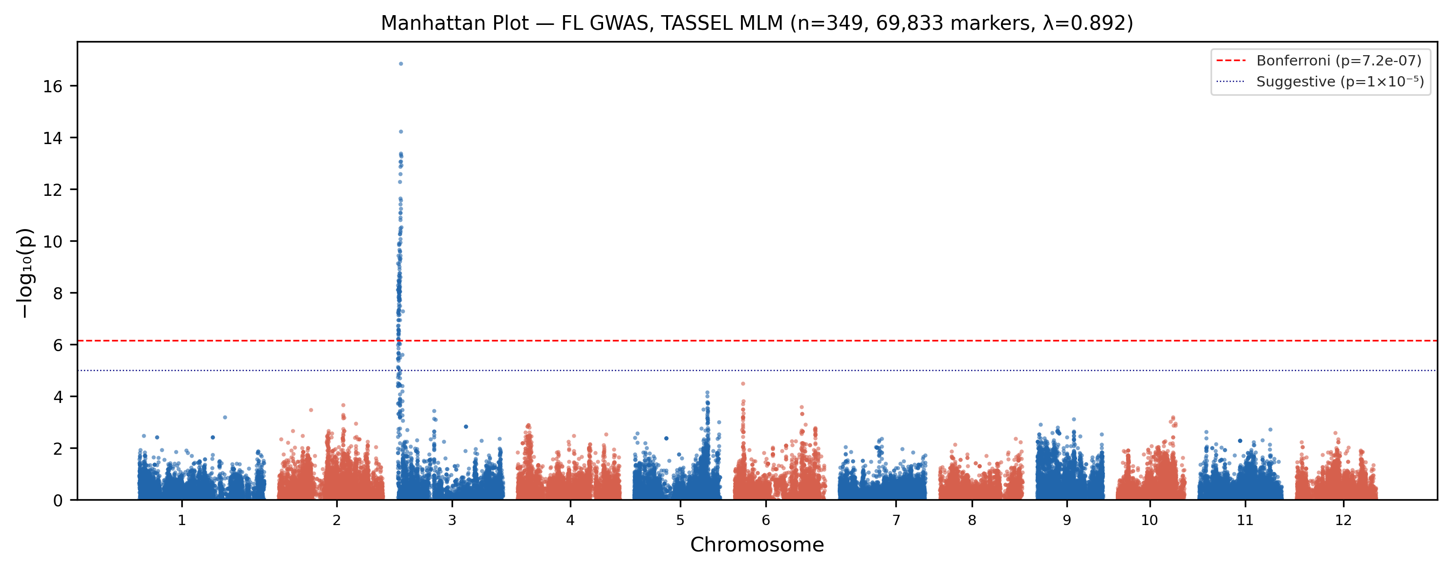
119 significant markers point to one broad chromosome 3 region
All 119 Bonferroni-significant markers and all 157 markers at BH FDR < 0.05 lie on chromosome 3. Lead SNP S3_1269941 has reported p = 1.41 × 10⁻¹⁷.
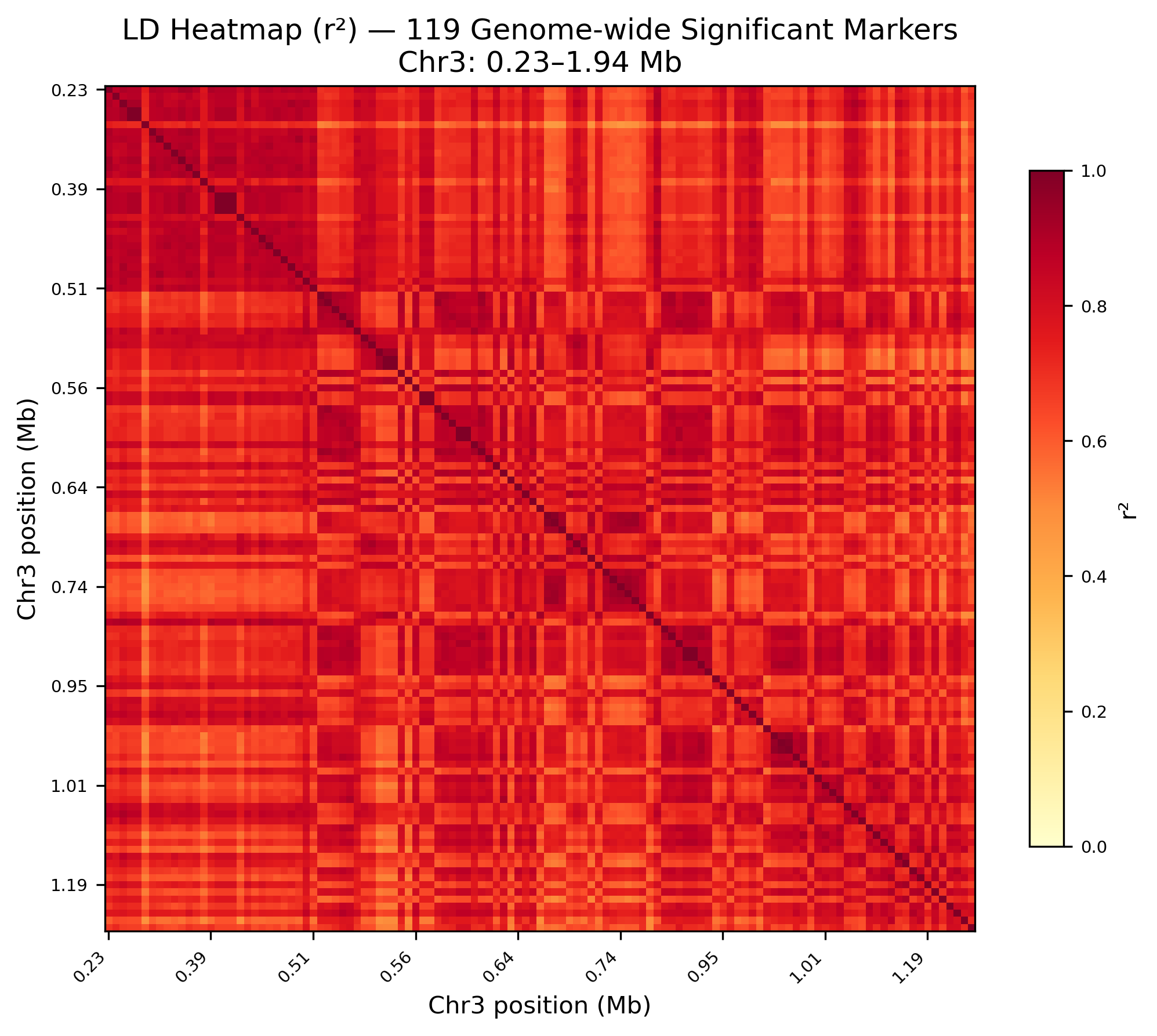
The significant interval spans Chr3:234,156–1,935,861 bp. Mean pairwise r² among significant markers is 0.740, supporting one major correlated association region; this does not prove a single causal variant.
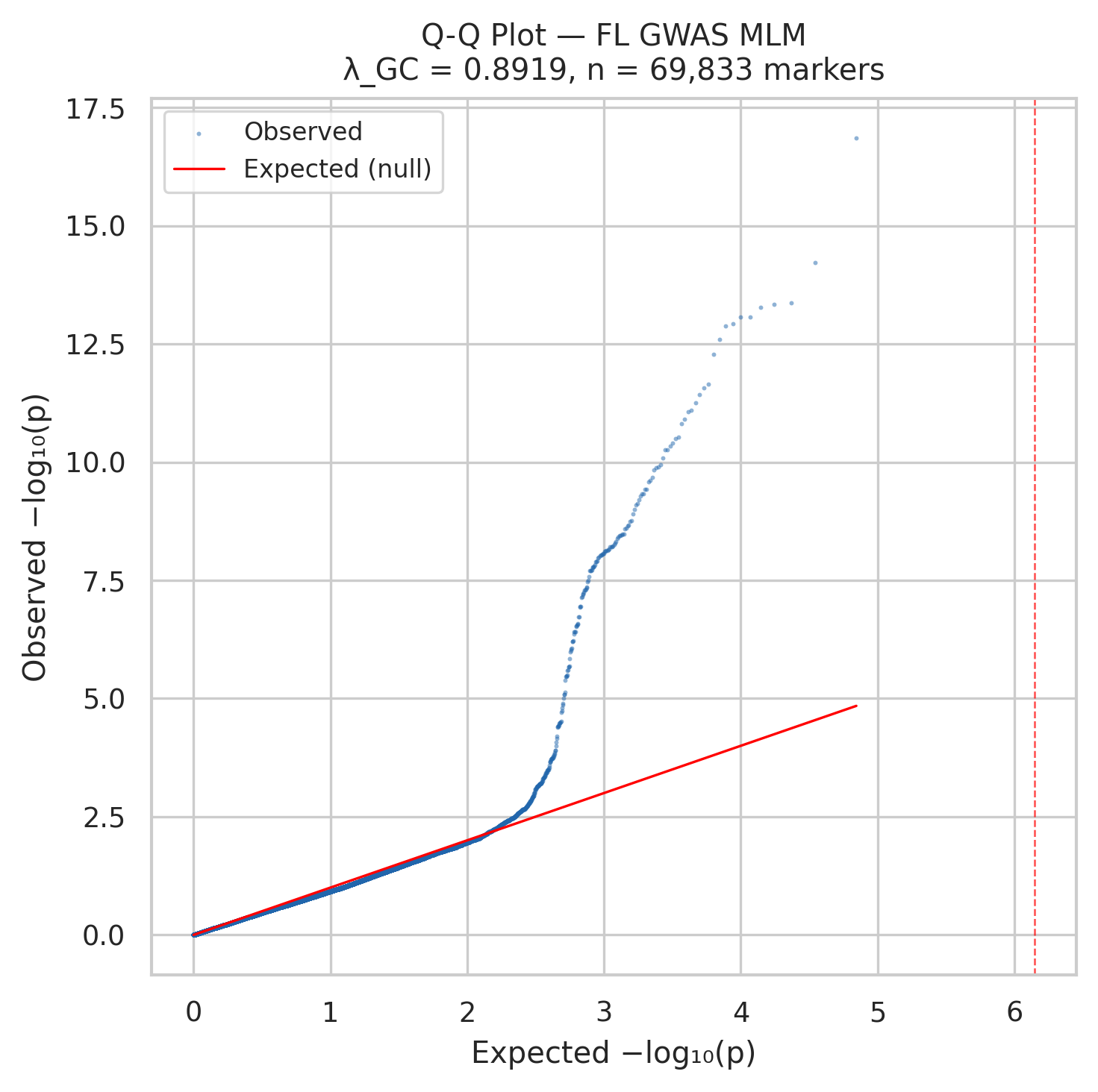
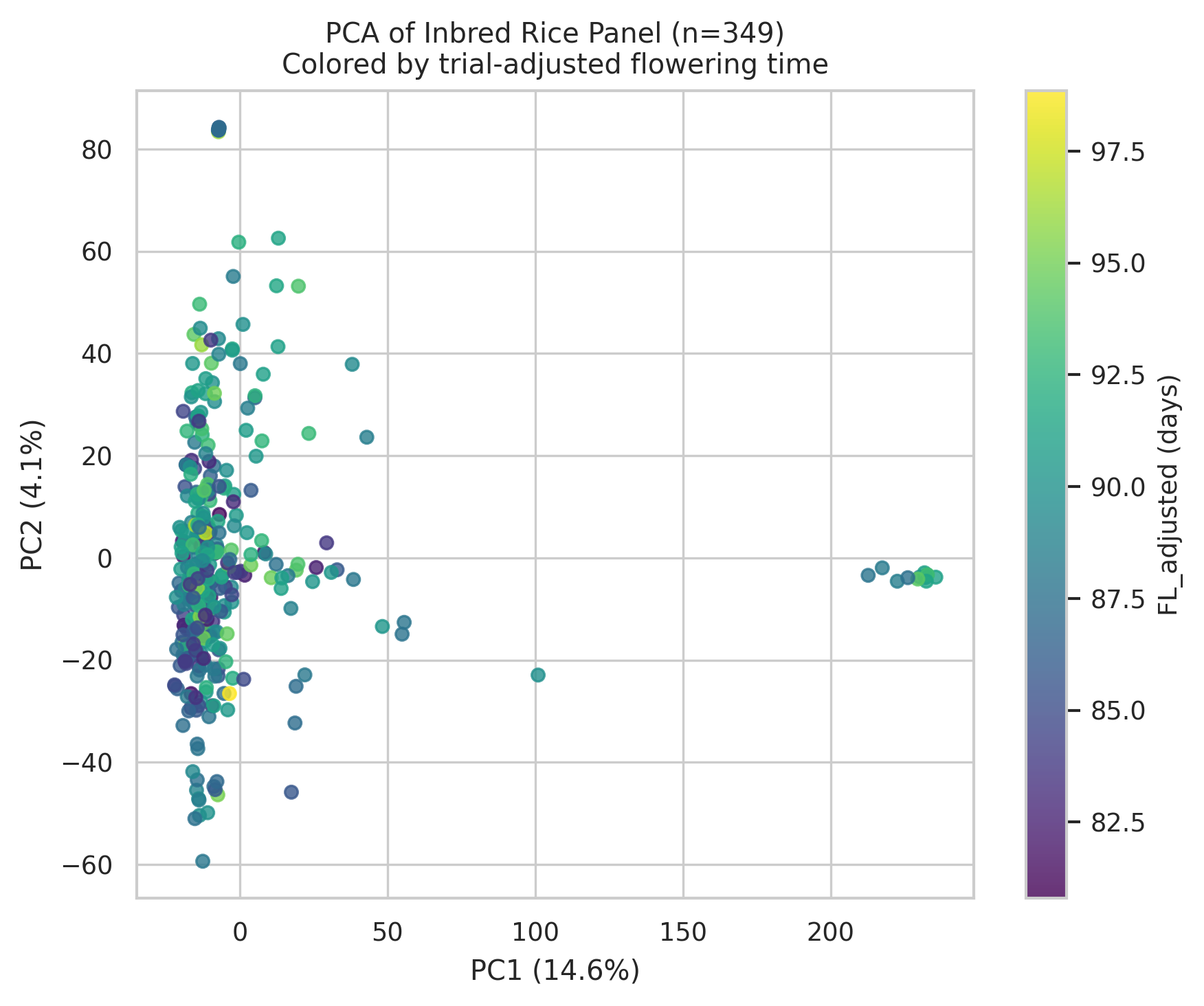
PC1 and PC2 explain 14.6% and 4.1% of genotypic variance in the report. GWAS λGC = 0.892 is below one, consistent with conservative calibration and possible loss of power; it does not establish that confounding is absent.
The fitted variance table assigns 60.7% to genotype and 26.4% to genotype × environment. Only 111 of the 349 lines were observed in all eight trials, making adjustment and uncertainty relevant to interpretation.
The lead marker overlaps LOC_Os03g03070, linked to OsMADS50
In the report's MSU v6.0 coordinates, S3_1269941 at Chr3:1,269,941 lies within LOC_Os03g03070 (1,268,854–1,270,781, minus strand). The downloaded annotation describes a putative expressed transcription factor. The interval contains 275 annotated genes; 53 genes directly overlap significant markers.
The session's final discussion identifies the OsMADS50 connection. The FunRiceGenes record lists LOC_Os03g03070 under OsMADS50 / OsSOC1 / DTH3, alongside LOC_Os03g03100 and published flowering-time studies. This is additional gene-identity context, not a replacement for the MSU v6.0 coordinates used in the analysis.
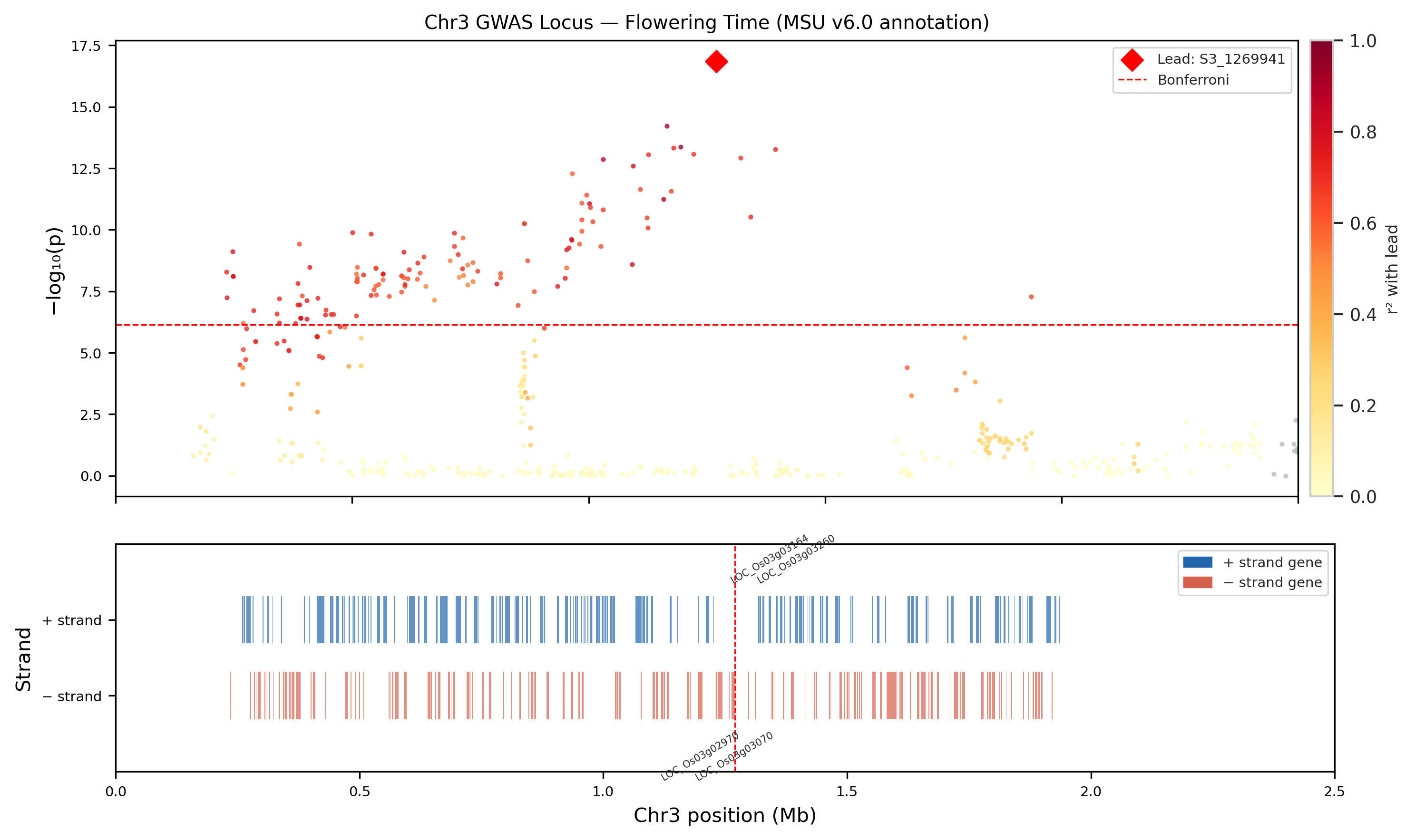
Known gene identity makes this a biologically relevant candidate region. The present GWAS does not establish that variation in OsMADS50 causes the flowering-time differences in this panel, identify a causal allele, or supply an independently validated selection marker.
Imputation, trial imbalance, and reporting gaps remain visible
- Imputation accuracy was not independently assessed; filtering at MAF 5% also limits rare-variant discovery.
- The trial design is unbalanced, and genotype × environment variation remains important. Environment-subset association sensitivity is a proposed follow-up, not an established result.
- The 1.70 Mb interval and strong LD cannot distinguish one causal variant from several linked effects. Independent-panel replication is absent.
- Allele-effect direction and magnitude are not provided in the canonical association output described by the report.
- The PDF methods report 5,799 analyzed plot records, while the output inventory describes 5,803 rows in plot_data_qc.tsv. The exported PDF alone does not resolve this discrepancy.
- The interpretation paragraph's claim that genotype plus G×E explains 95% conflicts with its variance table (60.7% + 26.4% = 87.1%). This page uses the component table and does not repeat the 95% claim.
- This case study was prepared from the supplied session PDF and its embedded figures. The underlying analysis artifacts were not supplied for an independent rerun or numerical audit.
Analysis artifacts documented in the session
The PDF lists the following outputs. They document the session's intended audit trail; the website provides the report and selected embedded figures, not separate downloads of the underlying tables or model objects.
qc_exclusion_ledger.jsonSample and marker exclusions, with sample_qc.tsv and the cleaned HapMapmet_model.rdsFitted phenotype model, alongside fl_variance_components.tsv and fl_blup_full.tsvflowering_time_adjusted.tsvLine-level phenotype input for GWASgwas_results_canonical.tsvFull 69,833-marker association table, with gwas_validation.json and significant-marker outputchr3_r2_matrix.npyLocal LD matrix, with region markers and ld_region_summary.jsonchr3_locus_candidate_genes.tsvRegional MSU v6.0 candidates, with annotated significant markers and reference checksums in msu_v60_reference_manifest.json